K-Means Clustering and Reading Groups
- gina2805
- Dec 28, 2022
- 5 min read
As someone interested in statistics, I've started shifting towards machine learning (ML). One of the simplest methods is through unsupervised learning, where the categories are unknown and are learned from the structure of the data.
In this post I'll explore K-Means clustering, an unsupervised ML method that creates categories based on features of data.
The dataset I'll use is from my dissertation (finally published earlier this year!). This dataset includes reading-related measures of vocabulary knowledge, reading experience, The Readers' Approaches to Text Questionnaire (TReAT-Q), and reading comprehension. Does the data make a distinction simply between "good" and "poor" readers? Or are there other categories?
Let's find out!

1. Overview
I'll walk through an R example of K-means clustering. It is possible to do this with Python (numpy, pandas, scikit-learn packages).
Below is the step-by-step of how I wrangled the data and ran the algorithm.
1. Overview
The goal of this RMD is to practice K-Means clustering with existing data. Data comes from Calloway et al. (2022) - “A measure of individual differences in readers’ approaches to text and its relation to reading experience and reading comprehension”.
I won’t go too into the details, but the purpose of the manuscript was to develop a measure that would be sensitive to distinguishing readers with different approaches to texts, including intrinsic and extrinsic motivators along with reading strategies.
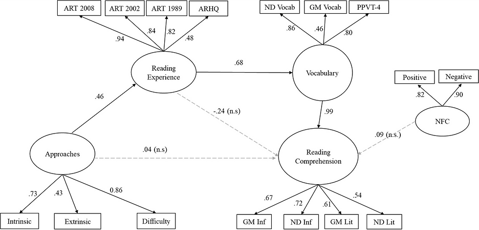
Along with the measure, reading-related measures of vocabulary, reading experience, and reading comprehension were taken and entered into a structural equation model.
The data for the current project can be found here:
Data file: Study2 >> “Study2_DATA_Formatted_for_SEM.csv”
There are 178 rows of data (i.e., 178 participants). The dataset is on the small side for K-means clustering, but let’s go with it for now.
1.1 Data description and preprocessing
Let's read-in the data! I used RMD for this, so that is the format I'll include the code in. This assumes that the .rmd file is in an "Analysis" folder and the data we want is in a separate "Data" folder.
```{r load.data}
reading_dat <- read.csv("../Data/Study2_DATA_Formatted_for_SEM.csv")
```
Before we get into implementing the ML algorithm, the first step is to do some processing of the data. Because all of the measures are on different scales, we'll first want to normalize the data.
Usually, one would do some type of exploratory factor analysis (EFA) or confirmatory factor analysis (CFA) to determine what variables are important for the latent factors (along with a structural equation model [SEM]). However, the Calloway et al. (2022) article did just that, so we'll be taking those findings, using the weights between the observed variables and their latent constructs, to establish the features to use for K-Means clustering.
The above paragraph assumes some knowledge of factor analyses, but it's not needed to work through this problem. The main thing to understand is that multiple measures related to reading were administered to young adults, and similar measures (e.g., three different measures of vocabulary) are thought to represent a latent factor. We essentially want to reduce the number of features that we use for the ML algorithm, going from 14 to 4.
The following columns will be used and fall under one of four latent factors.
Vocabulary
Gmac_Vocab - Gates McGinitie Vocabulary measure
ND_Vocab - Nelson-Denny vocabulary measure
PPVT_Std - Peabody Picture naming Vocabulary Test
Reading Comprehension
GM_Reading_Inference_P - Gates McGinitie Reading Comprehension test inference questions
GM_Reading_Literal_P - Gates McGinitie Reading Comprehension test literal questions
ND_Inference_P - Nelson-Denny Comprehension test inference questions
ND_Literal_P - Nelson-Denny Comprehension test literal questions
Reading Experience
ART_1989 - author recognition test, 1989 version
ART_2002 - author recognition test, 2002 version
ART_2008 - author recognition test, 2008 version
RH_totalz - zscored response to an average of 7 questions associated with readers’ recent reading history
The Readers’ Approaches to Text Questionnaire (TReAT-Q)
extrinsic_sub - subset of the TReAT-Q related to extrinsic reading motivation
enjoy_sub - subset of the TReAT-Q related to intrinsic reading motivation
diff_sub - subset of the TReAT-Q related to a desire for reading difficult or complex texts
Trim data and keep only relevant columns
```{r trim.data}
keep.cols <- c("PPVT_Std", "Gmac_Vocab", "ND_Vocab", "ART_1989", "ART_2002", "ART_2008", "ND_Inference_P", "ND_Literal_P", "GM_Reading_Inference_P", "GM_Reading_Literal_P", "extrinsic_sub", "diff_sub", "enjoy_sub")

read_trim <- reading_dat[,keep.cols]
```
Normalize Data
Normalize the data using the `scale()` function. Across all participants, normalizes so that each mean = 0 and the SD = 1.
```{r transf.data}
read_trimz <- scale(read_trim)
read_trimz <- as.data.frame(read_trimz)

# Add some additional columns that we didn't z-score (not that RH_totalz was already normalized)
read_trimz$Gender <- reading_dat$Gender
read_trimz$RH_totalz <- reading_dat$RH_totalz # don't want to Z-score this
read_trimz$Age <- reading_dat$Age
```
Assign weights
Assign weights to use for each of our latent factors. One could simply average the scores together, but due the the SEM that was originally done, we already know that some individual measures (i.e., observed variables) should have a higher weight than others.
Weights are from Calloway et al. (2022)
```{r weights.data}
# TReAT-Q
int_weight = 0.73
ex_weight = 0.43
diff_weight = 0.86

# Vocabulary
NDv_weight = 0.86
GMv_weight = 0.46
PPVT_weight = 0.80

# Reading comprehension
GM_inf_weight = 0.67
GM_lit_weight = 0.61
ND_inf_weight = 0.72
ND_lit_weight = 0.54

# Reading experience
ART_1989_weight = 0.82
ART_2002_weight = 0.84
ART_2008_weight = 0.98
RH_weight = 0.48

## Create new variables w/ the weights
read_trim_w <- read_trimz %>%
  mutate(weighted_NDv = (ND_Vocab*NDv_weight), weighted_GMv = GMv_weight*Gmac_Vocab, weighted_PPVT=PPVT_weight*PPVT_Std,

        weighted_GMlit = GM_lit_weight*GM_Reading_Literal_P, weighted_GMinf=GM_inf_weight*GM_Reading_Inference_P, weighted_NDlit = ND_lit_weight*ND_Literal_P, weighted_NDinf=ND_inf_weight*ND_Inference_P,

        weighted_ART89=ART_1989*ART_1989_weight, weighted_ART02=ART_2002*ART_2002_weight, weighted_ART08=ART_2008*ART_2008_weight, weighted_RH=RH_weight*RH_totalz,

        weighted_int=int_weight*enjoy_sub, weighted_ext=ex_weight*extrinsic_sub,
        weighted_diff = diff_weight*diff_sub)

# Create weighted average
# Vocab
read_trim_w <- mutate(read_trim_w, vocab=rowMeans(select(read_trim_w, c(weighted_NDv:weighted_PPVT)), na.rm=TRUE))

# Comp
read_trim_w <- mutate(read_trim_w, comp=rowMeans(select(read_trim_w, c(weighted_GMlit:weighted_NDinf)), na.rm=TRUE))

# Experience
read_trim_w <- mutate(read_trim_w, exp=rowMeans(select(read_trim_w, c(weighted_ART89:weighted_RH)), na.rm=TRUE))

# TReAT-Q
read_trim_w <- mutate(read_trim_w, treatq=rowMeans(select(read_trim_w, c(weighted_int:weighted_diff)), na.rm=TRUE))


# Keep just the last 4 columns w/ the mutated data
kmeans_dat <- read_trim_w[tail(names(read_trim_w), 4)]

```
1.2 Show Correlations
```{r cor.matrix, dpi=300}
pairs(kmeans_dat[,1:4], pch = 19)

```
1.3 Determine Number of Clusters
Different methods to determine the number of clusters to use.
Code adapted from: http://www.sthda.com/english/articles/29-cluster-validation-essentials/96-determiningthe-optimal-number-of-clusters-3-must-know-methods/
# Elbow method
set.seed(123)
fviz_nbclust(kmeans_dat, kmeans, method = "wss") +
    geom_vline(xintercept = 3, linetype = 3)+
  labs(subtitle = "Elbow method")
# Silhouette method
fviz_nbclust(kmeans_dat, kmeans, method = "silhouette")+
  labs(subtitle = "Silhouette method")
# Gap statistic
# nboot = 50 to keep the function speedy.
# recommended value: nboot= 500 for your analysis.
# Use verbose = FALSE to hide computing progression.
set.seed(123)
fviz_nbclust(kmeans_dat, kmeans, nstart = 25,  method = "gap_stat", nboot = 50)+
  labs(subtitle = "Gap statistic method")
# Using indices
nb <- NbClust(kmeans_dat, distance = "euclidean", min.nc = 2,
        max.nc = 10, method = "kmeans")
Output (most of the graph outputs are not shown here, but I'm showing the main indices graph that takes the 30 different indices and visually shows the number different indices that suggest each cluster.
## *** : The D index is a graphical method of determining the number of clusters.
##                 In the plot of D index, we seek a significant knee (the significant peak in Dindex
##                 second differences plot) that corresponds to a significant increase of the value of
##                 the measure.
##
## *******************************************************************
## * Among all indices:
## * 10 proposed 2 as the best number of clusters
## * 8 proposed 3 as the best number of clusters
## * 2 proposed 6 as the best number of clusters
## * 1 proposed 8 as the best number of clusters
## * 1 proposed 9 as the best number of clusters
## * 1 proposed 10 as the best number of clusters
##
##                    ***** Conclusion *****
##
## * According to the majority rule, the best number of clusters is  2
##
##
## *******************************************************************
Visualize Clusters
It looks like 2 clusters is our target. But Let's visualize 2-4 clusters as an example.
# Two clusters
k2 <- kmeans(kmeans_dat, centers = 2, nstart = 25)

# Three clusters
k3 <- kmeans(kmeans_dat, centers = 3, nstart = 25)

# Four clusters
k4 <- kmeans(kmeans_dat, centers = 4, nstart = 25)

# Visualize Clusters
fviz_cluster(k2, data = kmeans_dat); fviz_cluster(k3, data = kmeans_dat);
fviz_cluster(k4, data = kmeans_dat)


Show 2D plots
Sticking with the 2-cluster options, let's take a look at the different combinations of the four features as grouped by the two clusters.
As shown in the figures below, both the vocabulary and the reading experience features most easily show the distinction between the two clusters.


Comments